
Summary
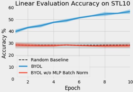
(1) BYOL often performs no better than random when batch normalization is removed, and
(2) the presence of batch normalization implicitly causes a form of contrastive learning.
These findings highlight the importance of contrast between positive and negative examples when learning representations and help us gain a more fundamental understanding of how and why self-supervised learning works.
The code used for this post can be found at https://github.com/untitled-ai/self_supervised.
Why does self-supervised learning matter?
Machine learning is typically done in a supervised fashion: we use a dataset consisting of the inputs and “right answers” (outputs) to find the best function that maps from the input data onto the right answers. By contrast, in self-supervised 1 learning, no right answers are provided in the data set. Instead, we learn a function that maps the input data onto itself (ex: using the right half of an image to predict the left half of an image).
This approach has proven successful in everything from language to images and audio. In fact, most recent language models, from word2vec to BERT and GPT-3, are examples of self-supervised approaches. More recently, this approach has had some incredible results for audio and images as well, and some believe that it may be an important component of human-like intelligence. This post focuses on self-supervised learning for image representations. For more background on self-supervised learning, see the resources below 2.
State of the art in self-supervised learning
Contrastive learning
Until BYOL was published a few months ago, the best performing algorithms were MoCo and SimCLR. MoCo and SimCLR are both examples of contrastive learning.
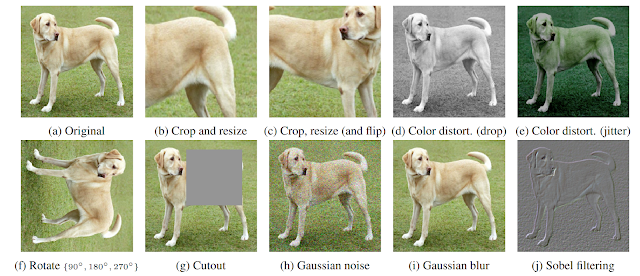
Contrastive learning is the process of training a classifier to distinguish between “similar” and “dissimilar” input data. For MoCo and SimCLR specifically, the classifier’s positive examples are modified versions of the same image, while negative examples are other images in the same data set. For example, suppose there is a picture of a dog. In that case, the positive examples could be different crops of that image (see below figure), while the negative examples could be crops from entirely different images.
BYOL: self-supervised learning without contrastive learning? Not exactly.
While MoCo and SimCLR use contrastive learning between positive and negative examples in their loss functions, BYOL uses only positive examples in the loss function. At first glance, BYOL appears to be doing self-supervised learning without contrasting between different images at all. However, it appears that the primary reason BYOL works is that it is doing a form of contrastive learning—just via an indirect mechanism.
To more deeply understand this indirect contrastive learning in BYOL, we should first review how each of these algorithms works. See Appendix A for a table that shows the notation used in each of the papers. In this post, we use the notation from BYOL for consistency.
SimCLR
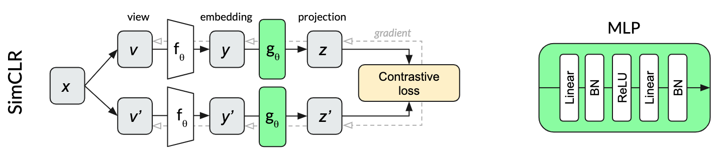
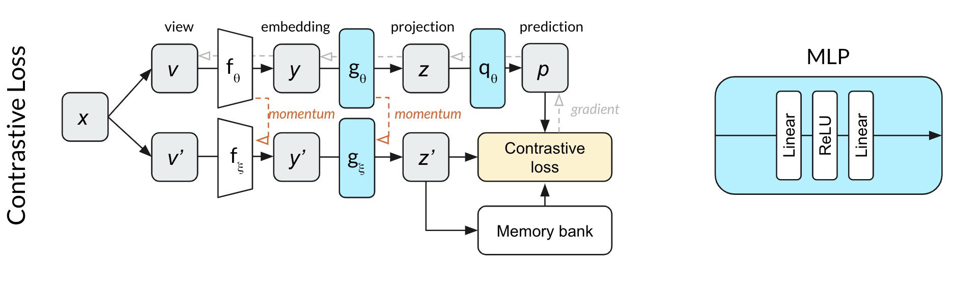
SimCLR is a particularly elegant self-supervised algorithm that managed to simplify previous approaches to their essential core and improve upon their performance. Two transformations v and v’ of the same image x are fed through the same network to produce two projections z and z’. The contrastive loss aims to maximize the similarity of the two projections from the same input while minimizing the similarity to projections of other images within the same mini-batch. Continuing our dog example, projections of different crops of the same dog image would hopefully be more similar than crops from other random images in the same batch.
The multilayer perceptron (MLP) used for projection in SimCLR uses batch normalization after each linear layer.
MoCo
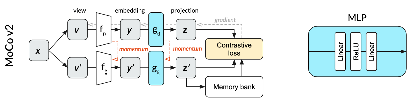
Relative to SimCLR, MoCo v2 manages to both decrease the batch size (from 4096 to 256) and improve the performance. Unlike SimCLR, where the top and bottom row in the diagram represent the same network (parameterized by ), MoCo splits the single network into an online network (top row) parameterized by and a momentum network (bottom row) parameterized by . The online network is updated by stochastic gradient descent, while the momentum network is updated based on an exponential moving average of the online network weights. The momentum network allows MoCo to efficiently use a memory bank of past projections as negative examples for the contrastive loss. This memory bank is what enables the much smaller batch sizes. In our dog image illustration, the positive examples would be crops of the same image of a dog. The negative examples are completely different images that were used in past mini-batches, projections of which are stored in the memory bank.
The MLP used for projection in MoCo v2 does not use batch normalization
BYOL
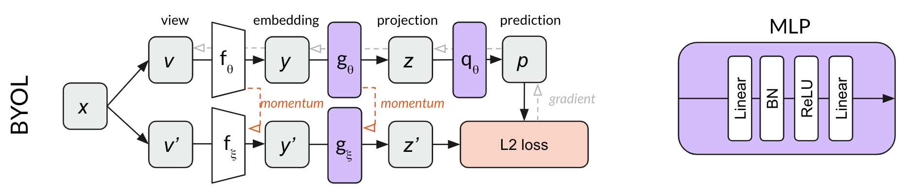
BYOL builds on the momentum network concept of MoCo, adding an MLP to predict z’ from z. Rather than using a contrastive loss, BYOL uses the L2 error between the normalized prediction p and target z’. Using our dog image example, BYOL tries to convert both crops of the dog image into the same representation vector (make p and z’ equal.) Because this loss function does not require negative examples, there is no use for a memory bank in BYOL.
Both MLPs in BYOL use batch normalization after the first linear layer only.
By the above description, it appears that BYOL can learn without explicitly contrasting between multiple different images. Surprisingly, however, we found that BYOL is not only doing contrastive learning, but that contrastive learning is essential to its success.
Our surprising results
We originally implemented BYOL in PyTorch using code we had written for MoCo. When we began training our network, we found that our network performed no better than random. Comparing our code to another available implementation (thanks sthalles!), we discovered we were missing batch normalization in the MLP. We were quite surprised that batch normalization was critical to training BYOL, while MoCo v2 did not require it at all.
For our initial testing, we trained a ResNet-18 with BYOL on the STL-10 unsupervised dataset using SGD with momentum and a batch size of 256 3. See Appendix B for details on data augmentation. Below are the first ten epochs of training for the same BYOL algorithm with and without batch normalization in the MLPs.
Why did this happen?
To investigate the cause of this dramatic change in performance, we performed some additional experiments.
Because the prediction MLP q changes the network depth compared to MoCo, we wondered if batch normalization might be needed to regularize this network. That is, while MoCo does not require batch normalization, it could be that MoCo does require batch normalization when paired with an additional prediction MLP. To test this, we started training the network shown above with a contrastive loss function. We found that the network was able to perform significantly better than random within ten epochs. This result made us suspect that something about not using a contrastive loss function causes the dependence of training on batch normalization.
We then wondered whether another type of normalization would have the same effect. We applied Layer Normalization to the MLPs instead of batch normalization and trained the network with BYOL 4. As in the experiments where MLPs had no normalization, the performance was no better than random. This result told us that the activations of other inputs in the same mini-batch are essential in helping BYOL find useful representations.
Next, we wanted to know whether batch normalization is required in the projection MLP , the prediction MLP , or both. Our experiments showed that batch normalization is most useful in the projection MLP, but the network can learn useful representations with batch normalization in either MLP. A single batch normalization layer in one of the MLPs is sufficient for the network to learn.
Performance for each variation
| Name | Projection MLP Norm | Prediction MLP Norm | Loss Function | Contrastive | Performance 5 |
|---|---|---|---|---|---|
| Contrastive Loss | None | None | Cross Entropy | Explicit | 44.1 |
| BYOL | Batch Norm | Batch Norm | L2 | Implicit | 57.7 |
| Projection BN Only | Batch Norm | None | L2 | Implicit | 55.3 |
| Prediction BN Only | None | Batch Norm | L2 | Implicit | 48 |
| No Normalization | None | None | L2 | None | 28.3 |
| Layer Norm | Layer Norm | Layer Norm | L2 | None | 29.4 |
| Random | — | — | — | None | 28.8 |
To summarize the findings so far: in the absence of a contrastive loss function, the success of BYOL training hinges on something about a single batch normalization layer related to the activations from other inputs in the mini-batch.
Why batch normalization is critical in BYOL: mode collapse
One purpose of negative examples in a contrastive loss function is to prevent mode collapse6. An example of mode collapse would be a network that always outputs [1, 0, 0, 0, …] as its projection vector z. If all projection vectors z are the same, then the network only needs to learn the identity function for in order to achieve perfect prediction accuracy!
The importance of batch normalization becomes clearer in this context. If batch normalization is used in the projection layer , the projection output vector z cannot collapse to any singular value like [1, 0, 0, 0, …] because that is exactly what batch normalization prevents. Regardless of how similar the inputs to the batch normalization layer, the outputs will be redistributed according to the learned mean and standard deviation. Mode collapse is prevented precisely because all samples in the mini-batch cannot take on the same value after batch normalization.
Batch normalization causes a similar effect in the prediction MLP. The function cannot learn the identity function if the mini-batch inputs are very similar: the batch normalization will redistribute the activations through vector space so that the final layer predictions are all very different. This function will only be successful at predicting projection vectors z’ if those vectors z’ are sufficiently well separated in representation space (that is, not collapsed) because the predictions p are constrained to be well separated across the mini-batch.
Why batch normalization is implicit contrastive learning: all examples are compared to the mode
Our findings seem consistent with a simple conclusion: one way to prevent mode collapse is to identify the common mode between examples. Batch normalization identifies this common mode between examples of a mini-batch and removes it by using the other representations in the mini-batch as implicit negative examples. We can thus view batch normalization as a novel way of implementing contrastive learning on embedded representations.
Said another way, with batch normalization, BYOL learns by asking, “how is this image different from the average image?“. The explicit contrastive approach used by SimCLR and MoCo learns by asking, “what distinguishes these two specific images from each other?” These two approaches seem equivalent, since comparing an image with many other images has the same effect as comparing it to the average of the other images. This equivalence is leveraged, for example, by prototypical contrastive learning.
Confirming our suspicions
Suppose the above is true (removing batch normalization causes BYOL to suffer from mode collapse). In that case, we should expect to see that all of the representations and projections (the , , and vectors) are equal — and that’s exactly what we saw.
We measured the cosine similarity of the first input projection vectors with the second input projection vectors after the training each of the variants above. We measured the average cosine similarity between the projections of positive examples (in blue), as well as the similarity to the projections from negative examples from the same mini-batch (in red) over each mini-batch in the tenth epoch of training.
With no batch normalization in or , the projections are highly aligned with both positive and negative examples (0.9999), indicating a collapse of the representation to a common vector. Because layer normalization does not introduce contrastive learning, it also results in aligned positive and negative representations. For standard BYOL training (i.e., using batch normalization), we get different vectors, as expected. The projections are more similar between the positive examples (0.88) than between negative examples (0.27).
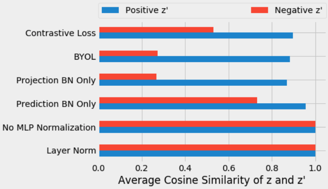
These results support our understanding of batch normalization as implicitly introducing contrastive learning using mini-batch statistics.
Additional experiments
Earlier batch normalization layers have the same effect (eventually)
So far, we had just looked at the first 10 epochs of training. When we trained for longer, we found that the batch normalization layers in the ResNet encoder had a similar effect to those in the MLPs. With batch normalization in the encoder (and not in the MLPs), the network first learned the function with collapsed representations, then gradually started to separate negative examples from positive ones.
Removing all batch normalization completely prevents learning—unless at least one technique is used to prevent mode collapse.
When we removed batch normalization from the ResNet encoder and trained the network using SGD, it was incapable of learning anything (for exactly the reasons we described above).
However, when we reached out to the authors, they kindly pointed out that we were not using exactly the same setup as in the original BYOL paper. By switching from SGD to layerwise learning rate adaptation (LARS) or adding weight decay, our network was able to learn again (though with significantly degraded performance).
We investigated each of these techniques and found that they were simply alternative methods for preventing mode collapse. Moreover, they were significantly less robust on their own—they depended on careful hyperparameter tuning, and without this tuning, they were prone to mode collapse and correspondingly terrible performance. Therefore, we concluded that batch normalization seems like the most robust technique for preventing mode collapse in BYOL.
Full discussions of those techniques, how they prevent mode collapse, and our additional experiments are included in Appendices C and D.
Conclusions
We find it quite interesting that even without negative samples in the loss function, batch normalization implicitly introduces contrastive learning in BYOL. This finding makes sense in hindsight—there is no learning when there is mode collapse, and batch normalization makes mode collapse impossible! Whether contrasting different images with each other or contrasting each image with the average of all images, a major part of learning is understanding how things differ from each other.
Besides shining a light on how batch normalization works in contrastive learning, this may serve as a lesson in how batch normalization can have unexpected side effects. With batch normalization, the network outputs are no longer learning a pure function of the corresponding inputs. For this and other reasons, it may be worth avoiding batch normalization in training. We suggest that other practitioners should perhaps default to alternatives like layer normalization or weight standardization with group normalization.
The opposite is an interesting avenue for future work as well. Rather than avoid batch normalization because of this implicit contrastive effect, it may be interesting to exploit that directly, allowing implicit contrastive learning at layers other than the final layer. One interesting open question is how much of batch normalization’s success in training neural networks is directly caused by this separation of internal representations.
Finally, we find it fascinating that BYOL can (with the right hyper-parameters) learn something even in the absence of either an explicit contrastive loss or an implicit contrastive mechanism via batch normalization. While we would not recommend that any practitioners use these networks in practice, we think they are a novel and interesting contribution to the field, and that their behaviors potentially provide a valuable glimpse into why some of these techniques (weight decay, weight standardization, and LARS) are so effective.
Given the rapid pace of progress in the field of self-supervised learning right now, new state of the art algorithms will surely be published soon. Please feel free to send us any relevant new results, and if there are any questions about our experiments or this blog post, don’t hesitate to reach out!
Thanks!
Thanks to our team members Bryden Fogelman, Timothy Devries, Hristijan Bogoevski, Bartosz Wróblewski, Jason Benn, Ali Rhode, and Kanjun Qiu for their feedback and comments. We also appreciate our friends Christina Kim, Benjamin Mann, Lisa Fetterman, William Levine, Andrey Zhmoginov, Chris Painter, Ian Thompson, Sarah Hong, Jeremie Harris, Vincent Chen, and Tom Brown who gave very helpful feedback. Finally, we are very grateful to the BYOL authors for reading this and giving us the opportunity to understand their algorithm better.
Appendix
For more details and data on our experiments, see the appendix to this post at the link above.
References
-
unsupervised is sometimes used interchangeably with self-supervised, though as Yann LeCun points out here, the term unsupervised is both loaded and confusing. ↩
-
for more on self-supervised learning, see DeepMind’s blog post, a practical overview from FastAI, or this in-depth post on everything related to self-supervised learning and representation learning. This GitHub repo contains many other relevant papers as well. ↩
-
The original BYOL implementation uses the LARS optimizer for 1000 epochs, with a batch size of 4096 and a warmup period of 10 epochs. See Appendices C and D for experiments around these and other hyper-parameters. ↩
-
because the only difference between using layer normalization and batch normalization is that the later is normalized across the other examples in the same mini-batch, while the former is independent of other examples. ↩
-
Linear evaluation accuracy on half of the STL10 test set, using the other half of the test set as training. We calculate the embeddings for the whole test set after each epoch and use an
sklearnlinear classifier to fit the data and calculate the accuracy. ��↩ -
collapsed representations is used with the same meaning in the BYOL paper (section 3). Other practitioners may identify the phenomenon as mode collapse. ↩